CDS 212, Homework 2, Fall 2010

1. REDIRECT HW draft

J. Doyle	Issued: 5 Oct 2010
CDS 212, Fall 2010	Due: 14 Oct 2010

Reading

• DFT, Chapters 3
• (FBS 9.1-9.3, 11.1-11.2)

Problems

1. [DFT 2.2, page 28]
   Consider the Venn diagram shown below, which relates the finiteness of norms (as described in DFT).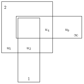
   

   Show that the functions defined below are contained in the locations shown in the diagram. All functions are zero for <amsmath>t < 0</amsmath>.

   1. <amsmath>\textstyle u_2 =\begin{cases} \frac{1}{t^{1/4}} \quad \text{if} \ t\leq 1 \\ 0 \quad \text{if} \ t> 1 \end{cases} </amsmath>
   2. <amsmath>\textstyle u_4 = 1/(1+t) </amsmath>
   3. <amsmath>\textstyle u_5 = u_2 + u_4 </amsmath>
   4. <amsmath>\textstyle u_9 = \begin{cases} 1 \quad t \in [2^{2k}, 2^{2k+1}],\, k = 0,1,2,\dots \\ 0 \quad \text{elsewhere} \end{cases}</amsmath>
2. Consider a second order mechanical system with transfer function <amsmath>

    \widehat G(s) = \frac{1}{s^2 + 2 \omega_n \zeta s + \omega_n^2}
   

   </amsmath>

   (<amsmath>\omega_n</amsmath> is the natural frequence of the system and <amsmath>\zeta</amsmath> is the damping ratio). Setting <amsmath>\omega_n = 1</amsmath>, write a short MATLAB program to generate a plot of the 2-norm as a function of the damping ratio <amsmath>\zeta > 0</amsmath>.

3. [DFT 3.1, page 44]
   Show that for a unity feedback system it suffices to check only two transfer functions to determine internal stability.
4. [DFT 3.2, page 44]
   Let <amsmath>

    \widehat P(s) = \frac{1}{10s + 1} \quad
    \widehat C(s) = k \quad
    \widehat F(s) = 1.
   

   </amsmath>

   Find the least positive gain <amsmath>k</amsmath> such that the following are all true:

   1. The feedback system is internally stable
   2. <amsmath>|e(\infty)| \leq 0.1</amsmath> when <amsmath>r(t)</amsmath> is the unit step and <amsmath>n = d = 0</amsmath>.
   3. <amsmath>\|y\|_\infty \leq 0.1</amsmath> for all <amsmath>d(t)</amsmath> such that <amsmath>\|d\|_2 \leq 1</amsmath> when <amsmath>r = n = 0</amsmath>.
5. [DFT 3.3, page 44]
   Consider a unity gain feedback system with <amsmath>r = n = 0</amsmath> and <amsmath>d(t) = \sin(\omega(t)) 1(t)</amsmath>. Prove that if the feedback system is internally stable then <amsmath>y(t) \to 0</amsmath> as <amsmath>t \to \infty</amsmath> if and only if <amsmath>\widehat P</amsmath> has a zero at <amsmath>s = j \omega</amsmath> or <amsmath>\widehat C</amsmath> has a pole at <amsmath>s = j\omega</amsmath>.
6. [DFT 3.4, page 44]
   Consider a feedback system with plant <amsmath>\widehat P</amsmath> and sensor <amsmath>\widehat F</amsmath>. Assume that <amsmath>\widehat P</amsmath> is strictly proper and <amsmath>\widehat F</amsmath> is proper. Find conditions on <amsmath>\widehat P</amsmath> and <amsmath>\widehat F</amsmath> for the existence of a proper controller such that
   1. The feedback system is internally stable.
   2. <amsmath>(y(t) - r(t)) \to 0</amsmath> when <amsmath>r</amsmath> is a unit step.
   3. <amsmath>y(t) \to 0</amsmath> when <amsmath>d = A \sin (100 t)</amsmath>.