|
|
| (9 intermediate revisions by 3 users not shown) |
| Line 10: |
Line 10: |
| This section contains a set of example that illustrate how the TuLiP code should be structured. This goes first so that we focus on the TuLiP interface and functionality and then figure out what is required to support it. | | This section contains a set of example that illustrate how the TuLiP code should be structured. This goes first so that we focus on the TuLiP interface and functionality and then figure out what is required to support it. |
|
| |
|
| === Load up an example stored in files and synthesize a controller ===
| | Notes from 14 May meeting: |
| This example shows how to load up a problem that is specified in files and synthesize a controller. Save the controller to a file, but also generate a version that can be executed in Ptolemy.
| |
|
| |
|
| ==== Code ====
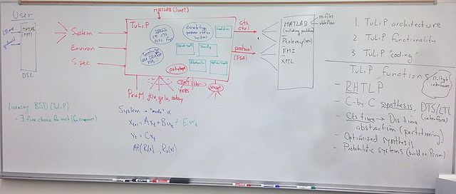
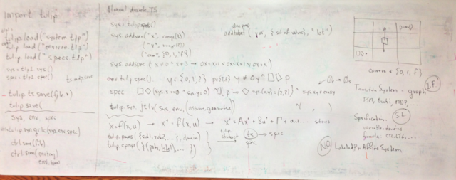
| | [[Image:tulip-planning_14May13.png|640px]] |
| <pre>
| |
| import tulip
| |
| | |
| # Load up the system and environment descriptions, plus specifications
| |
| system = tulip.ts.load("robot-discrete.tsf")
| |
| environment = tulip.sp.load("robot-env.spf")
| |
| specs = tulip.sp.load("robot-specs.spf")
| |
| | |
| # Synthesize a controller
| |
| controller = tulip.syn.jtlv(system, environment, specs)
| |
| | |
| # Save the controller in TuLiP and Ptolemy formats
| |
| tulip.ts.save("robot-control.tsf")
| |
| tulip.ptolemy.savefsm("robot-control.fsm")
| |
| </pre>
| |
| | |
| ==== Notes ====
| |
| # The <tt>.tsf</tt> (transition system file) and <tt>.spf</tt> (specification file) formats are the default TuLiP file formats.
| |
| #* Alternatively, perhaps we have a single file format <tt>.tlp</tt> and then use <tt>tulip.load</tt> and <tt>tulip.save</tt> to read and write. The type of object would just be part of the file specification. --[[User:Murray|Richard Murray]] ([[User talk:Murray|talk]]) 15:07, 11 May 2013 (PDT)
| |
| # The <tt>tf</tt> module contains data types and functions for representing different types of transition systems. Multiple transition systems are supported, including deterministic transition systems, Markov decision processes, Kripke structures, Rabin automata, etc.
| |
| # The <tt>sp</tt> module contains data types and functions for representing specifications. Multiple temporal logics, including LTL, MTL, CTL, PCTL, TCTL, STL, etc are supported.
| |
| # The <tt>syn</tt> module contains interfaces to various synthesis tools. Supported tools include JTLV, gr1c and PRISM. The input arguments must be compatible with the synthesis tool, but all arguments should be core TuLiP objects.
| |
| #* Would it make more sense to have a module for each program we support? So this line would become <tt>tulip.jtlv.syn</tt>? --[[User:Murray|Richard Murray]] ([[User talk:Murray|talk]]) 15:07, 11 May 2013 (PDT)
| |
| # The <tt>ptolemy</tt> module contains functions for interfacing with Ptolemy.
| |
| #* Should we instead make an FMI interface and then use Ptolemy's FMI capability? --[[User:Murray|Richard Murray]] ([[User talk:Murray|talk]]) 15:09, 11 May 2013 (PDT)
| |
| | |
| === Create a discrete example from scratch ===
| |
| | |
| This example shows how to create a system and environment from scratch, then synthesize a controller. It is based on the <tt>robot-simple.py</tt> example that is distributed with TuLiP and used in the EECI short course.
| |
| | |
| ==== Code ====
| |
| <pre>
| |
| import tulip
| |
| | |
| #
| |
| # Create the system transition system corresponding to a 2x3 grid of cells
| |
| #
| |
| system = tulip.ts()
| |
| system.addstates({'c11', 'c12', 'c13', 'c21', 'c22', 'c23'})
| |
| | |
| # Allow transitions between adjacent cells
| |
| system.addtransition('c11', True, {'c12', 'c21'})
| |
| system.addtransition('c12', True, {'c11', 'c13', 'c22'})
| |
| system.addtransition('c13', True, {'c12', 'c31'}})
| |
| system.addtransition('c21', True, {'c12', 'c22'})
| |
| system.addtransition('c22', True, {'c21', 'c23', 'c12'})
| |
| system.addtransition('c23', True, {'c22', 'c13'}})
| |
| | |
| # Add labels to selected points
| |
| system.addlabel('home', 'c11')
| |
| system.addlabel('lot', 'c13 or c23')
| |
| | |
| #
| |
| # Create an environment that allows an obstacle to move around in the same state space
| |
| #
| |
| # We model the environment in a slightly different way, just to show functionality
| |
| #
| |
| environment = tulip.ts()
| |
| | |
| environment.addvar('obs', system.states)
| |
| envspec = tulip.spec(environment,
| |
| ( obs = c11 -> next (obs = c12 or obs = c21) ) and
| |
| ( obs = c12 -> next (obs = c11 or obs = c13 or obs = c22) ) and
| |
| ( obs = c13 -> next (obs = c12 or obs = c31) ) and
| |
| ( obs = c21 -> next (obs = c22 or obs = c12) ) and
| |
| ( obs = c22 -> next (obs = c21 or obs = c23 or obs = c12) ) and
| |
| ( obs = c23 -> next (obs = c22 or obs = c13) )
| |
| ')
| |
| | |
| environment.addvar('park', {1, 0})
| |
| envspec = envspec + tulip.spec(environment, '[] <> !park')
| |
| | |
| #
| |
| # System specification
| |
| #
| |
| spec = tulip.spec({system,environment}, envspec + '->
| |
| (always eventually home) and
| |
| (always (park -> eventually lot)) and
| |
| (always !(
| |
| (obs = c11 and c11) or
| |
| (obs = c12 and c12) or
| |
| (obs = c13 and c13) or
| |
| (obs = c21 and c21) or
| |
| (obs = c22 and c22) or
| |
| (obs = c23 and c23) ) )
| |
| ')
| |
| | |
| # Synthesize the automaton
| |
| controller = tulip.syn.jtlv(system, environment, spec)
| |
| | |
| # Simulate the system
| |
| </pre>
| |
| | |
| === Discretize continuous dynamics ===
| |
| <pre>
| |
| import tulip
| |
| import control
| |
| | |
| # Create a hybrid system with 2D continuous space and no discrete dynamics
| |
| system = tulip.hybrid(2, {})
| |
| | |
| # Define the dynamics for the system
| |
| sysdyn = control.ss({{0,0,1,0}, {0,0,0,1}, {0, 0, 0, 0}, {0,0,0,0}}, {{0,0}, {0,0}, {1,0}, {0,1}}, {{1,0,0,0}, {0,1, 0,0}}, 0)
| |
| | |
| # Define the regions for the system, along with labels and dynamics
| |
| system.addregion({{0,0}, {1,1}}, 'c11', sysdyn)
| |
| system.addregion({{1,0}, {2,1}}, 'c12', sysdyn)
| |
| system.addregion({{2,0}, {3,1}}, 'c13', sysdyn)
| |
| system.addregion({{0,1}, {1,2}}, 'c21', sysdyn)
| |
| system.addregion({{1,1}, {2,2}}, 'c22', sysdyn)
| |
| system.addregion({{2,1}, {3,2}}, 'c23', sysdyn)
| |
| | |
| # Discretize the dynamics
| |
| tulip.discretize(system, 0.01)
| |
| </pre>
| |
|
| |
|
| == TuLiP classes == | | == TuLiP classes == |
|
| |
|
| === TransitionSystem ===
| | Notes from 23 May meeting: |
| | |
| A transition system consists of
| |
| * states - a list of elements that correspond to the states of the system. Elements are nominally strings
| |
| * transitions - optional subset of states x states indicating allowable transitions (doesn't have to be deterministic)
| |
| * actions - list of actions and what transitions they enable. If empty
| |
| * labels - list of atomic propositions for any subsets of states. Atomic propositions are given by set of all label outputs
| |
| * initial states
| |
| * acceptance sets - for Buchi and Rabin automata
| |
| | |
| Available functions
| |
| | |
| === Specification ===
| |
| A specification is a temporal logic formula. Specifications can be input and output as strings using the following symbols:
| |
| * state - evaluates to true if the system is in the discrete state
| |
| * atomic - evaluates to true if the atomic proposition is true
| |
| * logical operators: and, or, not, implies, &, ^, !, ->
| |
| * comparison operators: =, <=, >=, !=
| |
| * temporal operators: always, eventually, until, next, [], <>, U, X
| |
| * path operators: forall, exists, F, E
| |
| * probability operators?
| |
| | |
| === HybridSystem ===
| |
| | |
| The HybridSystem class is used to define systems that have continuous time dynamics. The state space of a hybrid system can be continuous, discrete or both.
| |
|
| |
|
| A space system consists of
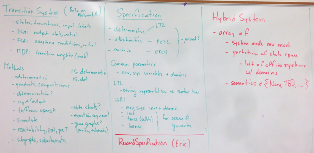
| | [[Image:tulip-planning_23May13.png|640px]] |
| * discrete state space - set of discrete states
| |
| * continuous state space - list of polygonal regions that are each subsets of R^n
| |
| * discrete inputs - set of discrete inputs that affect evolution of the system
| |
| * continuous inputs - set of continuous inputs that affect evolution of the system
| |
| * discrete transitions - set of guarded commands
| |
| * continuous dynamics - for each polygonal region, a set of dynamics that define the evolution of the system (given values for the inputs)
| |


